Using Deep Learning to Predict Water Point functionality from an Image
An essential part of ensuring that people have equitable access to services is being able to quickly and continuously assess whether those services are functioning properly. If your government provides health care it needs to know those clinics are open, if it provides public bus services it needs to know those buses are running on time, and if it provides water access it needs to know that water is flowing.
By training a deep learning model we are able to predict, from an image, whether a water point is functional or not with around 80% accuracy. Analyzing network activations shows that the model appears to be identifying a latent structure in the images. Given this, we expect the prediction accuracy to increase as the dataset expands.

Introduction
We’re involved in ongoing research to build better (e.g. cheaper, faster, more accurate) ways to answers these service delivery questions on behalf of our partners. Towards that end we recently ran some experiments to see if we can use labeled datasets to predict, from only an image of a water point, whether that water point was functioning or not. This lets us create models which, given an input image, output a prediction of whether that water point is working or not working. A model like this can help governments, civic organizations, and other actors in the development sector in at least two ways:
- An enumerator can take a picture of a water point and see if the model predicts that it is working or not, thereby validating their work.
- We can run the model against a set of historical image data to see where the model disagrees with the recorded values, and use this to flag potentially inaccurate data.
Image classification using neural networks has a long history going back to Yann LeCun’s work using convolution neural networks for digit recognition with LeNet. Our specific task of boolean (yes or no) classification for generic images has also attracted a lot of attention, such as with Kaggle’s Dogs vs Cats challenge. There’s a more generic annual challenge to build models from labeled ImageNet data to classify image content as well as multiple objects within an image. More recently, Google’s AutoML now provides a higher-level UI for building an image classifier.
Learning Method
To assess whether the general problem of predicting categorical column values from images in our domain is feasible, we use neural networks to predict whether a water point is functional or not from an image of the water point. We performed this experiment on the water point dataset because we expect there to be a relationship between the water point images and their functional status, and because this model can provide utility to our partners. We started with the basic model described by Francois Chollet in Building powerful image classification models using very little data. We then extended this model by adding an additional convolutional layer, increasing the range of image transformations, and varying the type and parameters of the model optimizer.
To generate the inputs to the model we first split the dataset by type of water point and then built separate models for each type. The original images are 1,836 by 3,264 pixels in both portrait and landscape format. To prepare them for training we used the EXIF information to rotate them as needed and reduced the resolution to 150 by 150 pixels. Additionally, we used Keras’ image generator to add rotated, sheared, zoomed, width and height shifted, and horizontally flipped versions of the images. Considering only hand pump type water point images, we have 1,605 examples, which we divide into 400 validation images and 1,205 training images.

We experimented with a number of different dropout rates, optimizers, learning rates, and decay rates. We tested the optimizers Adam, AMSGrad, Adagrad, Adelta, Adamax, Nadam, and RMSProp using a coarse grid search over the learning rate and dropout proportion hyper-parameters [1, 3]. We evaluated learning rates from 10-3 to 10-5 and dropout proportions from 0.4 to 0.7.
Results
We found that a learning rate of 10-4 provided the best results. Nadam did not produce good results, but the other optimizers performed reasonably well, all leveling off after around 100 training epochs. A dropout proportion of 0.5 appeared to perform the best, with performance increasingly negatively affected farther from that value.

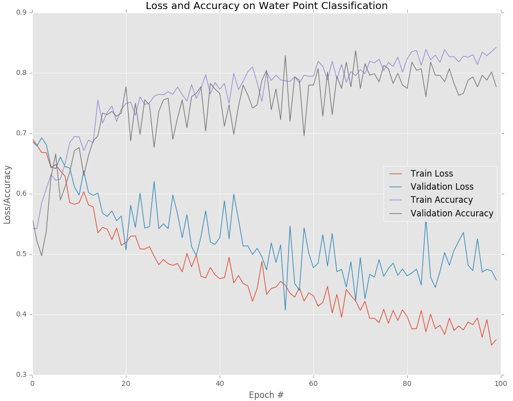
The above graph shows the loss and accuracy for the training and validation data over 100 epochs. With accuracy higher is better, whereas with loss lower is better. We see that over time both the training and validation set accuracies increase, while the losses decrease. This particular model was trained using the Adam optimizer with a learning rate of 10-4, dropout of 0.5, and batch size of 32. After 100 epochs the validation accuracy appears to have stabilized.
At the 100th epoch the training loss is 0.3572, training accuracy is 0.8433, validation loss is 0.4572, and validation accuracy is 0.7772. The validation accuracy measures how the model performs when evaluated on a set of images that it has never seen before. This is a useful proxy for how we would expect it to perform in the real world. We can therefore expect this model to correctly predict the functional status of around 80% of handpump waterpoint images.
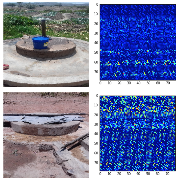
To gain insight into how the model is creating its predictions we will look at a couple of example classifications. The left hand column below shows scaled waterpoint images, and the right hand column shows the activation values for that image from a section of the neural network.

The model correctly predicts that the top image above is a functional water point and that the bottom image is not functional. In this model each image is given a score between 0 and 1, with 0 meaning the model is confident the waterpoint is functional, and 1 meaning the model is confident the waterpoint is broken. The top image received a score of 0.00774 and the bottom received a score of 0.907150.
The network activation images in the right-hand column above indicate greater activation through lighter colored pixels and vice versa. Network activation images are challenging to interpret, but the model seems to be using the existence of brown, muted colors as indicative of functional status. You’ll notice that in the top row, the brighter grass and blue bucket colors in the image appear inactive in the neural network. Alternatively, the large patch of beige parched land at the top of the bottom image leads to high network activation, as shown by the bright points at the top of that image’s activation graph.
Conclusion and Future Work
Along with increasing the number of samples to improve accuracy, there are potentially fruitful avenues to improve accuracy by increasing the amount of data in each sample. We can do this by adding existing organic data to the learning algorithm, e.g. location and time the image was taken, and by adding synthetic data, e.g. the population density at that location and time. Of course when expanding the input data it will be important to take into consideration the use case for the model and distinguish between what we can expect to know from what we are trying to predict.
There are also a number of improvements to the model that we can experiment with. The current hyper-parameters were chosen with a coarse grid search, we should do a fine grid search over the hyper-parameters and add additional hyper-parameters to the search space, including pool size and optimizer. We should experiment with additional network architectures, both deeper and wider. Given the complexity of the problem there’s good reason to believe our network cannot express the topological complexity of the dataset [2]. Although preliminary tests did not produce good results, we should also experiment further with transfer learning using pre-existing network weights, such as ImageNet.
This is only the start of an ongoing project and there are an exciting number of directions for future work. With these building blocks, we’re moving towards a toolset where creating a predictive model from your dataset is as easy as creating a chart.
A Python notebook for the model we used above is available in the dl4d repository. The image transformation code is a heavily modified version of Carin Meier’s Cats and Dogs With Cortex Redux.
If you are interested in exploring how machine learning can help address your needs please contact us at sales@ona.io.
Further Reading and References
- Duchi, Hazan, and Singer, Adaptive Subgradient Methods for Online Learning and Stochastic Optimization
- Guss and Salakhutdinov, On Characterizing the Capacity of Neural Networks using Algebraic Topology
- Kingma and Ba, Adam: A Method for Stochastic Optimization

